Recurrent Neural Networks (RNNs)

The classical RNN

Recurrent neural networks are a family of neural networks specialized for processing sequential data often of variable length. Unlike feedforward neural networks, RNNs share its parameters across data points and can thus easier scale to much longer sequences.

Mathematically, a recurrent neural network can be viewed as a function that calculates it’s state at time step recursively, i.e. in it’s most simple form by the equation: The intermediate states are usually referred to as hidden units of the network, which is why we denote them with henceforth. Since our goal is to process some input sequence , the module also usually uses to compute it’s hidden state , which can be written as A typical RNN will add additional architectural components such as output layers that read information out of the states to produce the final output. For example, if the task is to predict the next element in the sequence, we might add a linear layer to predict the next sequence element as .

Comparison to the Multilayer perceptron: If we compare a multi-layer perceptron with a RNN , the difference in equation becomes:

This has two major advantages:

1. The model always has the same input size, regardless of the input length
2. It is possible to use the same transition function with the same parameters at every time step This makes it possible to learn a single model that operates on all time steps and all sequence lengths rather than needing to train a separate model for all possible time steps.

What are the hidden units? When the recurrent network is trained on a task that requires predicting the future from the past, the network typically learns to use as a kind of lossy summary of the task-relevant aspects of the past sequence of inputs up to . Depending on the task, the model might decide to selectively keep some aspects of the past sequence, that are important for the final output, in higher precision than other aspects. For example when predicting stock prices, random fluctuations in the past might be less important to remember than the current overall trend (ascending / descending).

The different types of RNNs We present the 3 traditional types of RNNs:

1. RNNs that produce an output at each time step and have recurrent connections between hidden units: .
2. RNNs that produce an output at each time step and have recurrent connections only from the output at one time step to the hidden units at the next time step: . 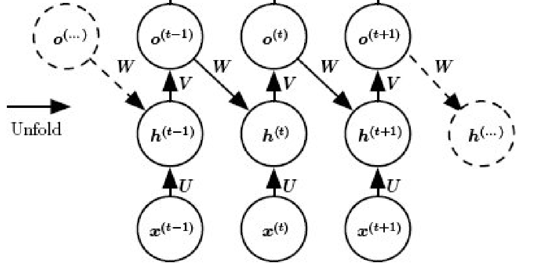 Image source: Deep Learning by Goodfellow, et al., Figure 10.4
3. RNNs with recurrent connections between hidden units that read an entire sequence and produce a single output. The model produces some hidden states using and then produces an output only from the final hidden state using some extra layers .

Example: A typical example is stock price prediction. Given the stock prices for the last 100 minutes we might want to predict what the stock price will be in the next minute . To do this, we can for example run the RNN to calculate and then add a linear layer that calculates the result: . After observing the real stock price at minute 101, we could again feed the sequence into the model to predict and so forth.

Further applications include:

• Time Series Forecasting: Beyond our stock price example, RNNs excel at predicting future values in sequential data - from weather forecasting and energy demand prediction to sales forecasting. The hidden state naturally captures trends and patterns over time.
• Natural Language Processing: Before transformers dominated the field, RNNs were the go-to architecture for:
  • Language Modeling: Predicting the next word in a sequence
  • Machine Translation: Encoding a sentence in one language and decoding it in another using encoder-decoder RNN pairs
  • Text Generation: Creating coherent text, from chatbots to creative writing
  • Sentiment Analysis: Understanding the emotional tone of text by processing words in context
• Speech Recognition and Synthesis: RNNs process audio signals frame by frame, making them natural fits for converting speech to text or generating human-like speech. Their ability to maintain context helps distinguish similar-sounding words.
• Music Generation: The sequential nature of music makes RNNs particularly suitable for composing melodies, harmonies, or even full musical pieces by learning patterns from existing compositions.
• Video Analysis: By processing video frames sequentially, RNNs can perform action recognition, video captioning, and anomaly detection in surveillance footage.
• Bioinformatics: RNNs analyze biological sequences like DNA, RNA, and proteins to predict structure, function, or identify patterns relevant to disease research.

While transformers have largely replaced RNNs in many NLP tasks due to their parallel processing capabilities and better long-range dependency handling, RNNs remain valuable for:

• Real-time processing where future context isn’t available
• Applications with strict memory constraints
• Tasks where the sequential inductive bias is beneficial
• Scenarios requiring online learning or continuous adaptation

Forward propagation in the classical RNN

Now we are going to look at the forward propagation equations for the classic RNN. It begins by specifying an initial state . Then for each time step in order to calculate the hidden unit , we simply apply linear layers to the input and the previous hidden unit , add them up and apply an activation function: Here denotes a bias term, are two matrices and is chosen as the activation function. To calculate the output , we apply another linear layer: If used in a classification task, we will usually regard the outputs as the output logits and then apply the softmax operation as a final post-processing step to obtain a vector of probabilities over all possible classes.

These equations are also often depicted using diagrams like these:

Backpropagation in the classical RNN

#todo

Example implementation

Now let us actually implement the classic RNN using PyTorch. We will write an autoregressive RNN that, given a sequence of text characters, predicts the next character in that sequence. The process will roughly look something like this: where we generate a new prediction and then afterwards feed it back into the model as the new input in order to generate the next prediction and so forth.

As always, we begin by setting up our PyTorch environment:

import torch
import torch.nn as nn
import torch.nn.functional as F
from torch.utils.data import Dataset, DataLoader
from torch.utils.tensorboard import SummaryWriter

device = 'cuda' if torch.cuda.is_available() else 'cpu'

We start by initializing the weights of the RNN as follows:

class RNN(nn.Module):
    def __init__(self, vocab_size, hidden_size, output_size):
        super().__init__()
        self.hidden_size = hidden_size
        self.embed = nn.Embedding(vocab_size, hidden_size)
        self.U = nn.Linear(hidden_size, hidden_size) # x -> h
        self.W = nn.Linear(hidden_size, hidden_size) # h -> h
        self.V = nn.Linear(hidden_size, output_size) # h -> o

Now we replicate the equations from the Forward propagation section:

class RNN(nn.Module):
	# ...
	
    def forward(self, x, h=None):
        x = self.embed(x)  # (B, T, H)
        B, T, _ = x.size()
        if h is None:
            h = torch.zeros(B, self.hidden_size, device=x.device)
        outputs = []
        for t in range(T):
            h = torch.tanh(self.W(h) + self.U(x[:, t, :]))
            out = self.V(h)
            outputs.append(out.unsqueeze(1))  # (B, 1, V)
        return torch.cat(outputs, dim=1), h  # (B, T, V), (B, H)

We allow passing a hidden state h to enable efficient continuation of predictions when new inputs come in. This allows the model to continue where it left off without needing to recalculate for the entire sequence. This is particularly valuable for our autoregressive generation process.

Here B represents the batch size, T the sequence length and H the hidden state dimension. Note that while our mathematical formulation shows a single bias term, the implementation uses two nn.Linear layers (self.W and self.U), each with their own bias. This is mathematically equivalent since two biases ​ combine to form a single effective bias

Next, we define our tokenizers. We start by loading some text from a file input.txt

with open("input.txt", "r") as f:
	text = f.read()

then generate the vocabulary:

chars = sorted(list(set(text)))
stoi = {ch: i for i, ch in enumerate(chars)}
itos = {i: ch for ch, i in stoi.items()}
vocab_size = len(chars)

and define our token encoder/decoders as follows:

def encode(s): return [stoi[c] for c in s]
def decode(t): return ''.join([itos[i] for i in t])

For generating text from the model, we define the following function:

def generate(model, start_str, length, device):
    model.eval()
    input_ids = torch.tensor(encode(start_str), dtype=torch.long)
    input_ids = input_ids.unsqueeze(0).to(device) # Model requires batch
    with torch.no_grad():
        _, h = model(input_ids) # Generate h for next token
        idx = input_ids[:, -1].unsqueeze(0) # Extract last token
		
        generated = start_str
        for _ in range(length):
			# Generate recursively h = f(h,x)
            logits, h = model(idx, h) 

			# Sample next token
            prob = F.softmax(logits[:, -1, :], dim=-1)
            idx = torch.multinomial(prob, num_samples=1)

			# Append generated character
            generated += itos[idx.item()]
    return generated

We can already try running it using:

print(generate(model, start_str="ROMEO:", length=200, device='cpu'))

Which e.g. may produce:

ROMEO:: J;PbI,-,$k
br$jPBN
cz?hniHaA xR'LD
xsuMbwjfW'wdULK!DJ$chKY!g!WauKXX
;CZQHWv krosHM JBfa:sAdVwgFuplL-$3Kxjx!
UEbeWIwgVm&ok-OsADgKY!&AX?Y.-hUuyX WjZgIaZLWU&xBP3DZ3TFVYuiyo:qxFLQX?DuqLEKVgkz-QyPHXTLFKJ

Now we continue with defining our dataset class. The dataset will not return single characters at a time, but instead return two entire blocks of size block_size that advance by one character at a time.

class CharDataset(Dataset):
    def __init__(self, data, block_size):
        self.data = data
        self.block_size = block_size

    def __len__(self):
        return len(self.data) - self.block_size

    def __getitem__(self, idx):
        x = self.data[idx : idx + self.block_size]
        y = self.data[idx + 1 : idx + self.block_size + 1]
        return x, y

Finally, we define the training loop.

data = torch.tensor(encode(text), dtype=torch.long)

def train_model(model, device, epochs=50):
    block_size = 128
    batch_size = 512
    train_loader = DataLoader(CharDataset(data, block_size), batch_size=batch_size, shuffle=True)
    optimizer = torch.optim.Adam(model.parameters(), lr=3e-4)
    loss_fn = nn.CrossEntropyLoss()

    model.to(device)
    global_step = 0
    for epoch in range(epochs):
        total_loss = 0.0
        total_grad_sq = 0.0
        for batch_idx, (xb, yb) in enumerate(train_loader):
	        xb, yb = xb.to(device), yb.to(device)
	        optimizer.zero_grad()
            
            logits, _ = model(xb)
            loss = loss_fn(logits.view(-1, logits.size(-1)), yb.reshape(-1))
            loss.backward()
            optimizer.step()

			# Logging
			total_loss += loss.item()
            grad_sq = sum((p.grad.data.norm(2).item() ** 2 for p in model.parameters() if p.grad is not None))
            grad_norm = grad_sq ** 0.5
            total_grad_sq += grad_sq
			print(f"Loss/Batch: {loss.item()}, {global_step}")
			print(f"GradNorm/Batch: {grad_norm}, {global_step}")
            
            global_step += 1
        print(f"Epoch {epoch+1}, avg loss: {total_loss / len(train_loader):.4f}")
        sample = generate(model, start_str="ROMEO:", length=200, device=device)
        print(f"Epoch {epoch+1}, generated text: {sample}")

If you run the training loop for long enough, you might actually see the problem of [[#What are the drawbacks of classical RNNs?|exploding/vanishing gradients]]:

GradNorm/Batch: 0.0800622015556688, 396
Loss/Batch: 2.2864320278167725, 397
GradNorm/Batch: 0.07994240105989828, 397
Loss/Batch: 2.290435314178467, 398
GradNorm/Batch: 0.0837944443319583, 398
Loss/Batch: 2.2783944606781006, 399
GradNorm/Batch: 0.08307291181557168, 399
Loss/Batch: 2.2832722663879395, 400
GradNorm/Batch: 0.08182225530517484, 400
Loss/Batch: 2.2813920974731445, 401
GradNorm/Batch: 0.08421354978431221, 401
Loss/Batch: 2.274799346923828, 402
GradNorm/Batch: 0.08386171047852181, 402

What are the drawbacks of classical RNNs?

1. Computation is very slow during training In contrast to [[Transformer]] models, RNNs do not posses a way to parallelize computation. RNNs process sequences sequentially, i.e. they must compute before they can compute , and so on. This creates a computational bottleneck: For a sequence of length , you need sequential steps that cannot be parallelized. On modern GPUs designed for parallel computation, this is highly inefficient.

   In contrast, Transformers compute attention between all positions simultaneously:

2. It is difficult for the model to access information from a long time ago, since the hidden state must remember all previous information that might be relevant

3. There is no way to consider future information. However bidirectional RNNs exist

4. Exploding/vanishing gradients Due to the repeated multiplication of weight matrices during [[#Backpropagation in the classical RNN|backpropagation]] through time, RNNs are highly susceptible to gradients becoming extremely large (exploding) or extremely small (vanishing), making training notoriously difficult. Exploding gradients can often be mitigated by clipping them to a maximal norm. However, vanishing gradients aren’t so easily fixed. [[Long short-term memory|LSTMs]] address this problem by introducing a dedicated ‘cell state’ and gating mechanisms. These allow gradients to flow more consistently across many time steps, as the cell state can be updated additively, preventing them from shrinking too quickly.

Some enhancements of the classical architecture include:

• [[Long short-term memory]]
• [[Gated Recurrent Unit]]

Deep Recurrent Network

Up until now, our model had just a single layer, which is usually not enough for complex tasks such as next token prediction. It would be better to stack multiple RNN blocks on top of each other, similar to stacking multiple [[Transformer]] blocks. The architecture remains largely the same, we just pass the input at time step through multiple linear layers, each maintaining their own hidden state , before arriving at the output . This way allows each layer to focus on a specific aspect of the sequence and maintain its own memory for that specific aspect.

This is how an implementation might look like:

class DeepRNN(nn.Module):
    def __init__(self, vocab_size, hidden_size, output_size, num_layers=2):
        super().__init__()
        self.hidden_size = hidden_size
        self.num_layers = num_layers
        self.embed = nn.Embedding(vocab_size, hidden_size)
        
        # Stack of RNN layers
        self.rnn_layers = nn.ModuleList([
            nn.ModuleDict({
                "W_ih": nn.Linear(hidden_size, hidden_size),
                "W_hh": nn.Linear(hidden_size, hidden_size)
            }) for _ in range(num_layers)
        ])
        
        self.W_out = nn.Linear(hidden_size, output_size)

    def forward(self, x, h=None):
        x = self.embed(x)  # (B, T, H)
        B, T, _ = x.size()
        
        # Initialize hidden state for each layer
        if h is None:
            h = [torch.zeros(B, self.hidden_size, device=x.device) for _ in range(self.num_layers)]
        
        outputs = []
        for t in range(T):
            inp = x[:, t, :]
            for l, layer in enumerate(self.rnn_layers):
                h[l] = torch.tanh(layer["W_ih"](inp) + layer["W_hh"](h[l]))
                inp = h[l]  # input to next layer
            out = self.W_out(h[-1])  # output from topmost layer
            outputs.append(out.unsqueeze(1))  # (B, 1, V)
        
        return torch.cat(outputs, dim=1), h  # (B, T, V), list of (B, H)

We can reuse the same training function from before:

if __name__ == "__main__":
    num_layers=8
    model = DeepRNN(vocab_size, hidden_size, vocab_size, num_layers).to(device)
    train_model(model, device)

---

Further Reading / Resources

• Deep Learning - Goodfellow, Bengio, Courville

• Predict Stock Prices Using RNN: Part 1